Understanding oscilloscope waveform thickness properties
The oscilloscope waveform shows the real electrical signal. When evaluating oscilloscope performance, you can examine its ability to display the same shape as the target signal. Assuming the oscilloscope has enough basic technical specifications - such as bandwidth, sample rate and equal frequency response, should the oscilloscope display a coarse or fine waveform better? The answer to this question is the same as most engineering questions: "depending on the situation ".
Now let's examine the properties of the oscilloscope and signals that help the user determine whether it is a coarse or a fine waveform. Two key attributes allow the user to understand the ability of their oscilloscope to display the target signal, which is the update rate and noise.
The effect of update rate on waveform thickness
The update rate represents the number of waveforms acquired, processed, and displayed by the oscilloscope in less than 1 second. The higher the update rate, the faster the oscilloscope can display the signal under test. The lower the update rate, the longer the oscilloscope will display the details associated with a particular waveform. Currently, the oscilloscope's update rate ranges from 1 million waveforms per second to 1 waveform per second. Simply change the oscilloscope settings and the same oscilloscope can display different speed ranges. The update rate is affected by multiple oscilloscope settings, including changing the depth of the acquisition memory, which can have a significant impact on memory depth.
Let's take a look at a simple example. The top half of Figure 1 shows an oscilloscope with equal bandwidth produced by two well-known manufacturers. The oscilloscope runs continuously and is connected to the exact same 10 MHz sine wave. One of the oscilloscopes shows a thicker waveform and the other shows a thinner waveform. This can result in different measured values. Which one is more accurate? One of the biggest differences between the two oscilloscopes is the update rate. Using the same settings, one of the oscilloscopes has an update rate of 1 million waveforms per second, which is 16,000 times faster than the update rate of the other oscilloscope.
How does this affect the waveform? The bottom half of Figure 1 shows how the two oscilloscopes connected to the same signal will be displayed when infinite persistence is turned on. Both oscilloscopes will build images of longer duration. After 10 seconds, the oscilloscope shows the same waveform shape and waveform thickness. In this case, the initial oscilloscope with a higher data rate can display a thicker waveform and more clearly represent the display content of each oscilloscope. By turning on infinite persistence, we can quickly evaluate.
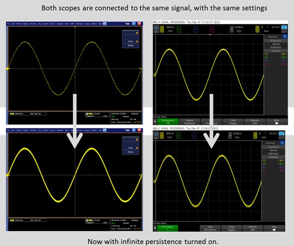
Figure 1. Two oscilloscopes with the same bandwidth and approximate noise are connected to the same signal. The noise of the two oscilloscopes is similar. The screenshot above shows the Tek DPO5104A, which has a very narrow waveform and provides more detail. The Agilent DSOX4104A displays a wider waveform. Why is there such a difference? The reason is the update rate. (Both scopes are connected to the same signal, with the same settings. The two oscilloscopes are connected to the same signal, using the same settings; Now with infinite persistence turned on. Now turn on infinite persistence.)
Turn on infinite persistence and wait 10 seconds. Both oscilloscopes display the same thickness. The Agilent oscilloscope has an update rate of 1 million waveforms per second, while the Tek oscilloscope has an update rate of only 60 waveforms per second in normal mode. The thickness of the waveform is related to the amount of noise added by the oscilloscope to the initial signal.
Effect of oscilloscope noise on waveform thickness
What is the accuracy of the oscilloscope measurement? Usually, from the perspective of the horizontal time base, the oscilloscope's measurement accuracy is extremely high, but from the perspective of the vertical time base, the accuracy is significantly reduced. What is the reason? One of the main reasons is the interference of noise on the measurement. The internal noise generated by the oscilloscope is coupled to the signal under test, resulting in signal convolution, which is digitized, stored, processed, and displayed in successive samples. The oscilloscope's analog-to-digital converter cannot distinguish between the noise generated by the oscilloscope and the noise generated by the actual target signal. However, you can run a simple test to determine how much noise your oscilloscope adds to the signal. Take a specific combination of settings to quickly determine how much noise your oscilloscope will produce and make a simple comparison between the two oscilloscopes.
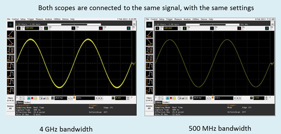
Figure 2. Two oscilloscopes with the same update rate are connected to the same signal. The thickness of the waveform displayed by the two is very different. What is the reason? The noise of a 4 GHz oscilloscope is higher than that of a 500 MHz oscilloscope. The reason for the difference in thickness is noise. (Both scopes are connected to the same signal, with the same settings, the two oscilloscopes are connected to the same signal, using the same settings)
Figure 2 shows two oscilloscopes looking at the same 10 MHz sine wave. One of the oscilloscopes shows a thicker waveform. According to the previous example, does the oscilloscope display a coarser waveform because of a faster update rate? The answer is no. Both oscilloscopes have the same update rate when turning on infinite afterglow, one of which will still display a coarser waveform and the other will show a thinner waveform. The difference is that one of the oscilloscopes has much higher noise than the other, and the noise difference produces a wider signal. Other sources of noise include active and passive probes located in the test setup. Active probes typically use a 50 Ω signal path in the oscilloscope channel that has less than 1 MΩ signal path noise.
How do you quickly learn how much noise an oscilloscope will generate? Most oscilloscope vendors will perform noise characterization on specific models and include these values ​​in the product literature. If the vendor does not provide it, you can apply for it or find it yourself. The measurement can be completed in a few seconds.
Disconnect all inputs from the front of the oscilloscope and set the oscilloscope to the 50 ? input path. You can also test on the 1M? path. Enabling the right amount of acquisition memory, 100Kpts to 1Mpts is sufficient. The oscilloscope enables infinite persistence to measure the height of the waveform. The thicker the waveform, the more internal noise the oscilloscope produces. The oscilloscope has a unique noise quality in each vertical setting. You can view the noise by observing the waveform thickness and quantify the noise with voltage AC true rms measurements for more analysis. Change the vertical setting to a more sensitive value - 100 mV to 10 mv/div - you can see the noise increase as a percentage of the full-scale vertical value, as shown in Figure 3.
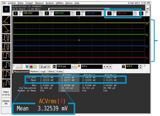
Figure 3. Quickly characterizing the oscilloscope's noise. Disconnect all inputs. Vrms AC measurements are made for the channels in each vertical setting.
If the initial signal is too narrow, the oscilloscope will reduce the noise and display a narrower waveform, resulting in better views and measurements. Change your oscilloscope settings to reduce bandwidth, thereby eliminating broadband noise that can cause signals to be too narrow. Oscilloscope vendors use a variety of methods to reduce the oscilloscope's inherent noise, such as averaging, high-resolution mode, and bandwidth limitations. The noise mitigation setting is ideal for oscilloscopes with low noise.
Target signal
The target signal can have both low noise and high noise. It is sometimes difficult to determine if the signal noise displayed on the oscilloscope is from the target signal or the internal noise of the oscilloscope. When the oscilloscope's ADC digitizes the signal, the ADC cannot distinguish between signal noise and oscilloscope internal noise. It saves the ADC output signal and displays the associated value. Can a coarser waveform represent your test signal or oscilloscope? There are several ways to get an answer. First, use the method mentioned above to quickly evaluate the internal noise of the oscilloscope. It is expected to add this bias at each sample point. Turn on infinite persistence and see if the waveform shape is thick or unchanged.
Interestingly, the infinite persistence also shows how the oscilloscope noise affects the target signal. Quickly test known waveforms and see how the oscilloscope waveform differs between normal display mode and infinite persistence mode, so you can easily understand the oscilloscope's noise and update rate. As shown in Figure 4, an oscilloscope with high noise and low update rate will initially display a fine waveform, which will generate a coarse waveform when infinite afterglow is turned on. An oscilloscope with high noise and high update rate will immediately display a coarse waveform - regardless of whether the signal being measured is narrow or wide. An oscilloscope with low noise and low update rate will initially display a fine signal. When the infinite persistence is turned on, the signal remains unchanged or thickens (if the target signal also produces noise). An oscilloscope with low noise and high update rate will display the target signal correctly at the beginning. When the infinite afterglow is turned on, the thickness of the displayed waveform remains unchanged.
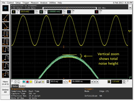
Figure 4. Enable the magnification math function to scale vertically above the waveform, and the user can determine the noise level of the signal by looking at the vertical range envelope (Vertical zoom shows total noise height).
The average mode generally thins the waveform by reducing the noise. The averaging mode allows the oscilloscope to perform continuous acquisitions, averaging each captured point, as shown in Figure 5. This method can reduce the overall noise of the oscilloscope by obtaining the average value of noise through multiple acquisitions. The mean tradeoff includes: the average method also calculates the average of the target signal values ​​and is only for repeated signals.
The high resolution mode reduces noise and allows the waveform to display the measured signal more clearly, as shown in Figure 5. This mode supports both repetitive and single capture signals. In high-resolution mode, the oscilloscope averages adjacent samples, thus reducing overall noise. One of the trade-offs to the high-resolution mode is that the oscilloscope must average the sample, and the resulting average sample point will appear less frequently than the initial sample point. This will reduce the effective sample rate and overall bandwidth.
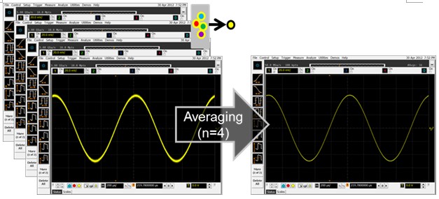
Figure 5. The average mode is for repetitive signals, which significantly reduces noise and provides accurate narrow waveforms [Averaging (n=4) average (n=4)].
Are you still thinking about the advantages and disadvantages of fine and coarse waveforms? You now have the expertise and technology to choose an oscilloscope that faithfully reproduces your target signal waveform. Or, you have selected an oscilloscope that you can use to determine how the oscilloscope displays a thin or coarse waveform of the signal under test.
Dog Treat Pouch,Pet Treat Pouch,Cat Treat Pouch,Leather Dog Treat Pouch
Ningbo Movepeak Pet Supplies Co.,LTD. , https://www.petsupplies-factory.com